Editor’s Note: Written by John Eargle, and republished courtesy of Harman Professional, this article is Chapter 2 of a book he co-authored with Chris Foreman entitled “Audio Engineering for Sound Reinforcement”. Eargle, who passed away in 2007, was JBL’s Vice President of Engineering for many years and became a well-known author and consultant. He was a skilled recording engineer responsible for more than 250 CD releases and his work in cinema sound brought him a Technical Oscar in 2001. Eargle’s many books on audio and acoustics are industry benchmarks and we are pleased to bring Pro Audio Encyclopedia readers this excellent introduction to psychoacoustics.
Introduction
Our ears do not always match our measuring instruments. We hear selectively, but we all hear very much alike. Apparent loudness is not the same as sound pressure level, but they are related. Perceived musical pitch is not the same as frequency, but they are also related.
There are many examples of sound masking: low pitched sounds tend to mask high pitched sounds, and loud sounds mask softer ones. In the time domain, early sounds tend to mask later ones if the two fall within a critical time interval.
In sound reinforcement we deal with psychoacoustics every day as we design systems that provide good musical balance, natural spatial relationships, and good speech intelligibility. It is essential to understand the basics of psychological acoustics, and that is the aim of this chapter.
Loudness Level
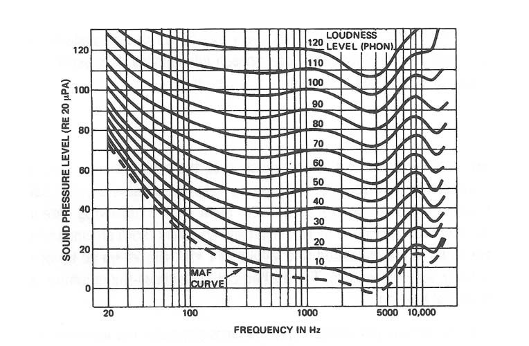
When you turn your stereo system down to a low playback level, the bass seems to drop off. If your system has a loudness control, you can restore some of the missing bass and achieve a better balance of highs and lows; or you can simply adjust the bass control as desired. What we are observing here are equal loudness level contours. The family of curves developed by Robinson and Dadson (1956) are shown in Figure 2-1. These curves (called phons) are equal to the measured SPL values at 1kHz. But as we go up or down in frequency the phon curves show a fairly wide divergence. The dashed curve indicates the minimum audible field (MAF) for young listeners with normal hearing.
In developing these curves, Robinson and Dadson tested a large population of listeners with normal hearing. The test subjects compared the apparent loudness of bands of noise centered at 1 kHz with noise bands at both higher and lower frequencies and noted the differences between them. Those differences were then compiled into the curves shown in the figure.
Here is an example of their use. Consider a sine wave at 1kHz at a measured SPL of 100 dB. By comparison, a 100-Hz tone will have to be about 3 dB higher in level to sound as loud as the 1 kHz tone. Now let’s make the same comparison at a level of 50 dB SPL. Here, the difference between 1 kHz and 100 Hz is 8 dB, indicating a total difference of 5 dB at 100 Hz when comparing the 50-phon and 100-phon curves.
If we make these measurements at 40 or 50 Hz we will find a divergence of about 12 dB with respect to1 kHz over the same range of 10 and 5 phons. This explains why subwoofers in music reinforcement and theater systems have to be specified in such great quantities; they simply have to be capable of playing that much louder in order to be perceived as keeping up with the midband.
We can see that in the motion picture theater, at peak reference levels per channel of 105 dB SPL, the subwoofers must produce between 115 and 120 dB in the 30 to 40 Hz range if they are to sound as loud as the midband.
Subjective judgments of loudness level
If you ask a person with normal hearing to make an estimate of “half loudness” or “twice loudness” of a wideband noise signal by adjusting the volume control of a comparator circuit, you will find that it takes approximately a 10-dB difference, louder or softer, to produce the subjective judgment of twice or half as loud. This may come as a surprise, considering that a 3-dB difference in level corresponds to twice or half power. It is no wonder then that we need such large amplifier and loudspeaker arrays for large reinforcement systems. If the sensation of loudness increases in a linear manner, then it takes an exponential progression in power amplifiers and loudspeakers to match it. Each time we increase the playback level by 10 dB, we have to increase both loudspeakers and amplifier output capability by a factor of 10.
Using the sound level meter to determine loudness levels
We discussed the SLM earlier in Chapter 1. In order to use the SLM effectively over a wide range of applications, we must take into account the ear’s relative insensitivity to low frequency signals at low levels. It is customary to incorporate into the SLM a set of weighting curves, such as those shown in Figure 2-2. The two important curves here are the flat curve and the A-weighted curve.
When making measurements of effective loudness level in the range below about 50 dB-SPL, it is customary to use the A-curve in order to get a reading that better corresponds to how the ear hears. You can see that the shape of the A-weighting curve is approximately the inverse of the 50-phon curve shown in Figure 2-1.
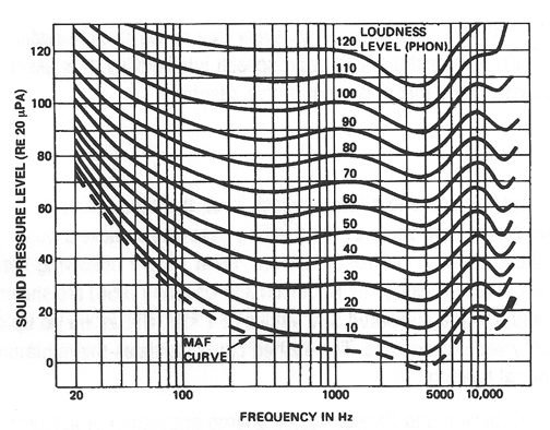
Figure 2-1: Robinson-Dadson Equal Loudness Contours
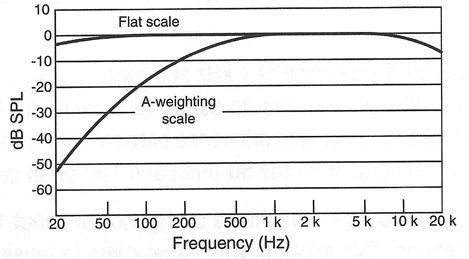
Figure 2-2: Standard Weighting Curves, A-Weighting and Flat Scales
The flat curve in the SLM is used for making all high-level acoustical measurements. As we will see in later chapters, A-weighting may also be used in making low-level noise measurements of electronics and microphones. The term dB(A) is generally used to indicate level measured with A-weighting.
Protect Your Hearing; Another Use for the A-Weighting Curve
As practitioners of sound reinforcement we may be subjected to fairly high sound pressure levels. Many people have abused their hearing over the years, and we are more conscious now of the need for self-imposed hearing conservation. In determining the deleterious effects of high-level noise, the A-weighting curve is used, since it relates directly to sound pressures that are present at the eardrum.
US Government permissible exposure to noise levels under OSHA (Occupational Safety and Health Act) regulations are:
Table 2.1 Permissible Noise Exposure Criteria
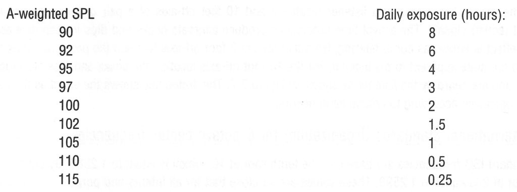
Many rock concerts routinely have A-weighted levels in the 110 to 115 range, and we know how long the exposure at a typical concert can be. The best advice we can give is to start taking care of your hearing while you are still young. If you are ever in doubt, wear ear defenders. For what it is worth, the EPA (Environmental Protection Agency) has set even more stringent standards than those shown above.
Loudness Dependence on Signal Duration
Short, impulsive sounds may not sound very loud as such, but their tendency to overload a system is just as pronounced as the same sound presented continuously. This general tendency is shown in Figure 2-3. Note that a signal which is only 2 msec long will sound approximately 15 dB lower in level than the same signal if it is presented for 200 msec or longer.
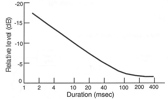
Figure 2-3: Signal Loudness Dependence on Duration
This fact has considerable influence on signal metering and what we want the meter to show us. For example, if a meter is intended to indicate program apparent loudness, we may not want it to respond strongly to program signals of very short duration. On the other hand, if we are operating a broadcast station, even very short signals can cause over modulation and interfere with a broadcaster on an adjacent channel. In this case we must be aware of instantaneous signal level at all times.
Critical Bandwidth
Although trained listeners can detect very small differences in the pitch of complex tones, we all have difficulty in detecting the pitch of pure tones that are closely spaced. We can do the following experiment which illustrates this: Take two sine wave oscillators and initially set them to the same frequency (say, 1 kHz); then, slowly change the frequency of one of them. At first you will hear a slow beating effect (equal to the difference in their frequencies), but you will still hear only a single tone.
As you continue moving the frequencies farther apart, you will eventually hear a sensation of roughness in the sound, and then you will begin to hear the two individual frequencies as such. The beating and roughness are now gone and the two tones will begin to sound smooth as the two frequencies move farther apart. Details here are shown in Figure 2-4.
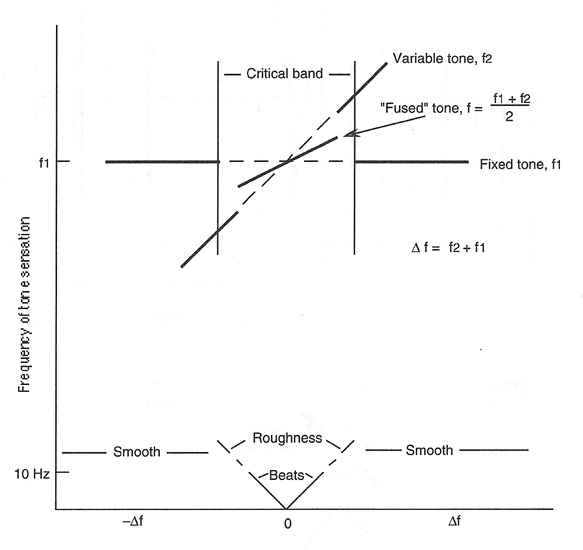
Figure 2-4: Critical Bandwidth, Definition
The frequency interval over which we will hear the single, fused tone is known as a critical band. Critical bandwidth varies over the audible spectrum, but over the range from 500 Hz and upward it is very close to a one-third octave. Below 500 Hz it tends to remain fairly constant, as shown in Figure 2-5.
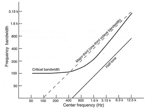
Figure 2-5: Critical Bandwidth Variation Over the Normal frequency Range
The critical band may be thought of as the fundamental pitch “information gathering” unit of hearing. For example, in making adjustments in sound system frequency response, equalizers operating at the ISO standard one-third octave centers are normally used, since our judgments of loudness are based on the total acoustical power within a critical bandwidth. In other words, it may not be necessary to use equalizers that cover smaller intervals than about one-third octave.
Combing or comb-filtering
Here is an example of critical bandwidth as it applies to normal sound reinforcement applications. Figure 2-6 shows the physical response at a listener located 2 and 10 feet off-axis of a pair of loudspeakers radiating coherent (equal) signals. The arrival time differences produce alternate peaks and dips in response as shown, and the effect is known as comb filtering. Note that for the 2-foot off-axis location the peaks and dips are fairly wide and are quite apparent to the listener. For the 10-foot off-axis location the peaks and dips are much closer together and are heard by the listener as shown at Figure 2-7. The dotted line shows the effect as the peaks and dips are perceived according to critical band hearing.
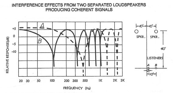
Figure 2-6: Development of Comb Filtering Due to Time Delays Between Loudspeakers
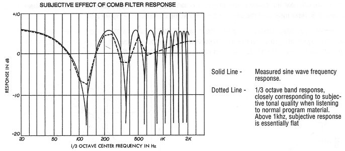
Figure 2-7: The Effect of Critical Bands on the Audibility of Comb Filtering
ISO (International Standards Organization) Third-Octave Center Frequencies
The standard ISO frequencies are based on the tenth root of 10, which is equal to 1.2589. By comparison, the third root of 2 is equal to 1.2599. These values are so close that for all intents and purposes we can consider them to be equal. The following chart shows the intervals of third octave frequencies over a range from 10 Hz to 20 kHz:
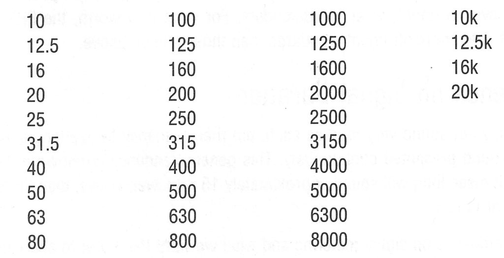
Note that these values have been rationalized; they are rounded off so that values never contain more than three significant figures. Examining the operating panel of a one-third octave audio equalizer you will typically find these series of frequencies covering the range from about 31.5 Hz to 20 kHz.
Localization Phenomena, Haas and Damaske
We can normally detect clearly the direction of any sound radiating from a single point. However, if two separated sources radiate the same signal, we will likely hear the sound as arriving only from the source that reaches our ears first. This is the so-called law of the first wavefront” and has been described in detail by Haas (1956).
Haas’ data is shown in Figure 2-8. If we have two loudspeakers that are radiating the same signal at the same level, but with one of them delayed 5 msec with respect to the other, as shown at A, the listener will clearly hear the sound arriving from the loudspeaker at the left. If the leading loudspeaker is reduced in level approximately 10 dB, we will hear the sound originating as a broad image from a point between the two loudspeakers, as shown in B. Haas measured the effect and arrived at the data shown in Figure 2-9.
As shown here, delays from zero up to 5 msec have a “trading value” with respect to level from zero to 10 dB for restoring the delayed signal to a neutral position between the two sources. For greater delays, from 10 msec up to about 25 msec, the 10 dB reduction of the earlier signal will suffice to keep the localization at a neutral position.
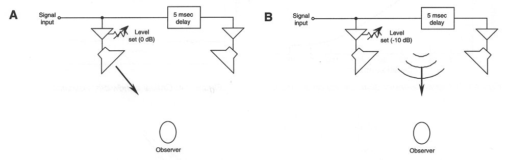
Figure 2-8: The Haas or Precedence Effect. Localization tends toward the earlier source (A): combination of level and delay time effects (B).
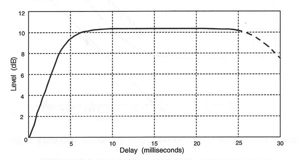
Figure 2-9: The Trading Value of Delay and Amplitude Differences Due to the Haas Effect
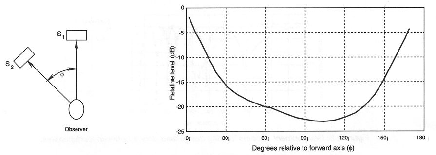
Figure 2-10: Binaural Masking Thresholds
The critical band may be thought of as the fundamental pitch “information gathering” unit of hearing. For example, in making adjustments in sound system frequency response, equalizers operating at the ISO standard one-third octave centers are normally used, since our judgments of loudness are based on the total acoustical power within a critical bandwidth. In other words, it may not be necessary to use equalizers that cover smaller intervals than about one-third octave.
At delays beyond about 25 msec the listener will begin to hear two separate sound sources, one as a slight echo after the other.
This phenomenon is often called the Haas effect, or more generally the precedence effect, and is of great value in both music and speech reinforcement. Through this effect, we can apply digital delay to sounds arriving from a nearer loudspeaker and thus “fool” the listener into localizing the apparent sound source in another direction. We will discuss this technique in more detail in later chapters dealing with specific applications.
Binaural Masking Thresholds – The Damaske effect
It has been observed many times that a dominant sound directly in front of a listener can mask an uncorrelated sound, such as noise, if it appears to come from the same frontal direction. However, if the uncorrelated sound is heard from another direction, particularly from the sides, it will be much more apparent to the listener. Damaske (1967) made the measurements shown in Figure 2-10. Here, the secondary uncorrelated sound is successively moved around the listener, and its level is adjusted so that it is just masked by the primary sound, which is stationary at the front.
When the secondary sound is presented from a bearing angle of 90°, it must be about 23 dB lower in level in order to be masked by the frontal signal.
The implications for stereo reinforcement are important: if stereo music is mixed down for presentation in mono, some important details which may be readily apparent in stereo presentation may be masked. System mixing engineers must be aware of this and prepared to make adjustments in the levels of individual secondary program components if music reinforcement is simultaneously done in surround sound, stereo, and mono.
General Requirement for Good Speech Intelligibility
Whether in amplified or unamplified speech presentation, the requirements of speech intelligibility are very much the same:
1. Speech loudness level. Average speech levels should be in the 65 to 70 dB range if persons with normal hearing are to understand it without effort. Under noisy conditions the speech level will have to be raised accordingly.
2. Speech signal-to-noise ratio. For ease in listening, average speech levels should be about 25 dB higher than the prevailing noise level. However, at elevated speech levels in noisy environments, a somewhat lesser speech-to-noise ratio is possible; typically, a 15-dB speech-to-noise ratio may suffice in sports activities where there is considerable spectator noise. This trend is shown in Figure 2-11.
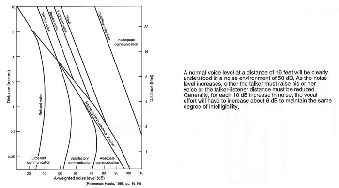
Figure 2-11: Required Communications Levels and Distances in the Presence of Noise
3. Reverberation time. Normal speech occurs at a rate of about three syllables per second; thus, a reverberation time of 1.5 seconds or less will not interfere with the normal perception of speech. Beyond critical distance in the room, the reverberation following each syllable will already have diminished by about 13 dB before the onset of the next syllable, and this will allow each succeeding syllable to be clearly heard. Reverberation time in this range may actually increase intelligibility through the increase in overall loudness; however, reverberation times longer than 1.5 seconds will progressively interfere with speech intelligibility. See the representation of this in Figure 2-12. In particular, distinct echoes in the 100 msec range or greater can be very deleterious to speech intelligibility.
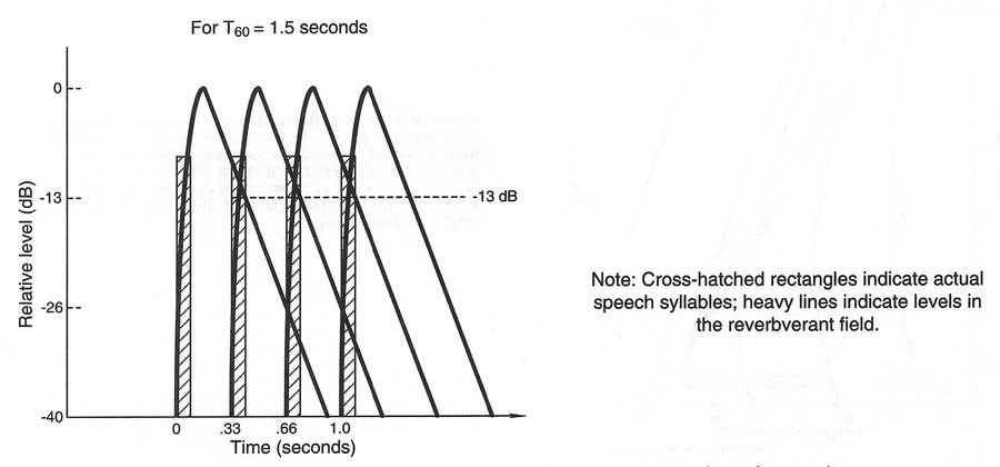
Figure 2-12: Effect of Reverberant Overhang on Perception of Speech
4. Uniform coverage. All listeners should be well within the range of the talker or of the loudspeaker reproducing the sound of the talker. All patrons in the audience should expect to hear accurately and comfortably.
5. Spectral integrity; freedom from distortion. In the specific case of reinforced speech it is essential that the voice spectrum (125 Hz to 4000 Hz) be reproduced with accuracy and that the transmission be substantially free of audible distortion.
Measuring Speech Intelligibility – Syllabic Testing
Speech intelligibility in a given environment is tested by using syllables imbedded in “carrier” sentences. The syllables are selected at random and are presented as follows by a talker speaking in a clear and natural manner:
“I want you to identify the word dog.”
“Now, please identify the word will.”
The test syllables are not to be stressed in any manner, and the purpose of the carrier sentence is to place the test syllable into the flow and tempo of normal speech, including any effects of room reverberation. Normally, if a listener can identify 85% of random syllables in a number of tests, then that listener will be able to understand about 97% of the words in normal speech context. Standard word lists are published by the ISO with instructions for their use.
Syllabic testing is a tedious procedure, but it is accurate. What speech reinforcement system designers want are relatively simple methods and procedures for predicting speech intelligibility, even if they have to give up some degree of accuracy. In a later chapter we will deal with some of the in situ test procedures that enable us to estimate the speech intelligibility in a space. We will also discuss some of the early prediction techniques that can be applied to construction jobs still on the drawing board.
We are by no means through with our discussion of intelligibility. Please refer to Appendix 5 for more detailed discussions of intelligibility measurement and estimation.