by Frederick J. Ampel and Ted Uzzle
For four centuries, natural philosophers and scientists have sought to quantify and derive qualitative standards for sound. Today’s technology enables investigations into the finest detail and structure of sound and audio signals. In order to understand today’s sophisticated computerized measurement systems and place their capabilities in perspective, it is useful to examine, from historical and scientific perspectives, the technological developments and systems that gave birth to the science of audio measurement.
At The Beginning
For centuries it was thought that sound was so ephemeral that any attempt to capture it — to hold a ruler against it — would be a fruitless exercise. In fact, until the 17th century natural philosophers thought it absolutely illogical to make any attempt to quantify it or even theorize about its measurement.
Aristotle (384-322BC), working from ancient researches into theater design, reasoned that high pitches must travel faster than lower pitches. The experimental means to disprove this theory were readily available, but no such experiments were performed for two thousand years, and even then experimenters withheld their contradictory results for fear of being spurned, ridiculed, or ostracized.
Even the word for this science cum art — acoustics — comes from elsewhere. It came to English from the French, to which there is a problematical derivation from the Greek. Francis Bacon (1561-1626) used it in his 1605 book Advancement of Learning. In 1863 an anonymous author in Philosophical Transactions of The Royal Society wrote, “Hearing may be divided into direct, refracted, and reflex’d, which are yet nameless unless we call them acousticks, Diacousticks, and catacousticks.” The word was needed because at precisely that moment natural philosophers (or scientists, as in the 19th century they would begin to style themselves) needed a word for the experiments they were beginning to conduct.
Finally, in the second half of’ the 17th century the invention of calculus created, almost overnight, a revolution in our understanding and study of sound propagation. Now we had formulas for densities and elasticities, displacements of strings, superposition and propagation, plates and shells — they march page after page after hundreds more pages and endless thousands of equations through Lord Rayleigh’s Theory of Sound. Yet, the one simple statement that sound does this or that was not forthcoming. The new mathematical techniques created a huge, powerful machine for processing and analyzing experimental results, but these exercises usually took place in a curious vacuum: there were no experimental results to test them against.
The Speed Of Sound
In prehistoric times people knew sound traveled more slowly than light. This was demonstrated every time a flash of lightning was followed by the crack of thunder. Later, a tree would be found exploded to bits and burnt to ash, locating the exact target of the lightning,
The earliest actual measurements were made by Pierre Gassendi (1592-1655) and Matin Mersènne (1588-1648). Mersènne used a pendulum to measure the time between the flash of exploding gunpowder and the arrival of the sound. Gassendi used a mechanical timepiece, and it was he who discovered that the high-pitched crack of a musket and the boom of a cannon arrived at the same time and realized that all pitches travel at the same speed.
In his 1687 book Prlncipia Mathematica, Newton predicted the speed of sound using the new calculus to create a purely mathematical analysis. Newton’s friends John Flamsteed (1646-1719; the first Astronomer Royal) and comet-discoverer Edmond Halley (1656-1742) measured the speed of sound to confirm Newton’s triumph. They watched through a telescope at the Greenwich observatory as a cannon was fired at Shooter’s Hill, three miles (4.8 km) away. To their utter mortification they found Newton’s prediction to be 20% slow.
They tried over and over, they attempted to account for every variable, they resurveyed the distance across the open fields, and still they could not get their measurement to agree with theory, Finally, unable to find a flaw in Newton’s theory and unable to account for their measurements, they abandoned the work while Newton held firmly to his published sound speed.
When multiple experiments could no longer be denied, Newton finally fudged the theory to produce the measured number. In his one foray into acoustics, the great god Newton behaved in a thoroughly dishonorable way.
In 1738 the Academy of Sciences in Paris measured and published a speed of sound within 0.5% of the value we accept today. After that, the French would lead the field in measurements of the speed of sound in solids. Jean Biot (1774-1862) measured the speed of sound in iron by assembling great lengths of newly cast iron water pipes and banging them with hammers. It was reported that Parisian public works officials would hold up pipe installations to permit this kind of scientific work.
Frequency Analysis
The Italian scientist, inventor, and experimentalist Galileo (1564-1642) drew a knife edge across the milled (or serrated) edge of a coin and noted the tone produced. He theorized sound to be a sequence of pulses in air. Sliding the knife more quickly produced higher tones, so he realized higher tones required a faster train of pulses.
In March 1676 the great British scientist Robert Hooke (1635-1703) described in his diary a sound-producing machine. Five years later he demonstrated it to the Royal Society. A toothed wooden wheel was rotated, and a card or reed was held against it. Children still do something like this today, with a playing card held against the spokes of a bicycle wheel. Hooke noted a regular pattern of teeth produced music-like sounds, while more irregular teeth produced something that sounded more like speech.
Hooke’s work wasn’t published for a quarter century (1705) and wasn’t used for further study for 150 years. However, by 1834 the Frenchman Félix Savart (1791-1841) was building giant brass wheels 82cm across, with 720 teeth. Savart’s contribution was a mechanical tachometer connected to the axis of the toothed wheel. He calibrated a rotational scale with the tooth rate, and for the first time demonstrated that specific tones were associated with specific frequencies (Figure 1).
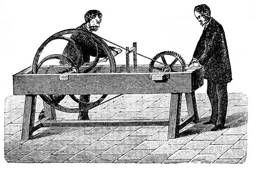
Figure 1. Savart’s wheel allowed frequencies heard in air to be compared with the buzz of the toothed wheel (1830).
He could determine the frequency of a tone heard in air by using his ear to match it with the toothed wheel and reading the frequency from the tachometer. He was using his ear and brain to do what a modern electrical engineer would call heterodyne analysis.
History is sometimes casual about assigning names. These great toothed wheels, the part invented by Hooke, are today called “Savart’s wheels,” while Savart’s having contributed the tachometer is forgotten.
In 1711 Britain a magnificent invention was made that would be elemental in it’s effect on acoustics, music, and medicine. So crucial was this device that in acoustics it would be the basis for two centuries of measurement. John Shore (1662-1752) was sergeant-trumpeter to George I, and magnificent music was composed for him by Henry Purcell (1659-1695) and Georg Fredrick Handel (1685-1759). Shore’s contribution to the science of measurement was the tuning fork — a frequency standard that was now available an that we can still refer to. Not realizing the impact of his work, Shore, with typical understatement and a touch of sarcasm, named his construct “the pitchfork”.
By the end of the 19th century Karl Rudolph Koenig (1832-1901) was building tuning forks with tines 8 feet long with a 20-inch (508 mm) diameter. Koenig built clocks that used ultra-accurate tuning forks to drive the escapement, a concept that would be incorporated into wristwatches a century later.
Looking At Sound Waves
In 1807 Thomas Young (1773-1829) coated a glass cylinder with lamp-black, pushed a pin through a flexible diaphragm, and by shouting into the diaphragm was able to see the sound waves scratched into the lamp-black. The Frenchman Édouard-Léon Scott de Martinville (1817-1879) elaborated on this idea. He used the ears of decapitated dogs as receiving horns to concentrate the sound waves. Across the small end of the ear he put a feather, whose sharpened tip “wrote” sound waves in the lamp-black on a cylinder. He demonstrated this in 1854, calling it the phonautograph (Figure 2). Later versions looked stunningly like Edison’s phonograph of 20 years later, although of course it could not play back.
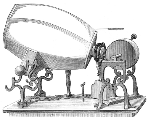
Figure 2. de Martinville’s phonautograph allowed experimenters to look at sound waveforms (1856).
Tuning forks became an industry, but the factories that were mass-producing them needed a quick and absolutely accurate way to compare a newly made fork against a standard. This can be done by ear, of course, but that is difficult in the noisy environment of a metalworking factory. In 1854 the Frenchman Jules Lissajous (1822- 1880) developed an optical method of great elegance.
Lissajous turned two forks at right angles to each other, so one vibrated horizontally and the other vertically. Lissajous would shine a spot of light onto a tine of one fork, reflect it onto the tine of the other fork, and observe the looping pattern through a lens system (Figure 3).
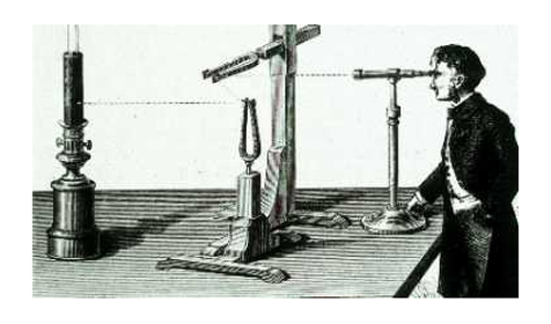
Figure 3. The mechanical oscilloscope developed by Jules Lissajous (1857).
Later he devised a way to project these patterns onto a screen. These patterns, named for Lissajous, revealed relative frequency, amplitude, and phase. Later Hermann Helmholtz (1821-1894) replaced one fork with a horn and reflective diaphragm, so the frequency of a fork could be compared with sounds captured from the air. The fork was what we would today call the timebase for what amounted to the earliest mechanical oscilloscope.
These mechanical devices would later be elaborated upon by Dayton Miller (1866- 1941), who called his device the phonodiek, and Maximilian Julius Otto Strutt, (1903-1992). In the 1920’s, Strutt was working for N. V. Philips in the Netherlands. He demonstrated the first chart recorder with ultrahigh writing speed. He used a further elaboration of Miller’s phonodiek,
This device, built for Strutt by Siemans and Halske of Germany, used a horn with a diaphragm at the small end, with a mirror on the diaphragm that would deflect with its vibrations. The optical system used a spot of light shining into this mirror, but this time the spot of light was captured by a moving ribbon of cinema film.
By using an appropriate lens, the deflection of the spot could be logarithmic. A later version used electromagnetic shutters developed for optical sound on film. Strutt made chart recordings on 35mm film of reverberative decays, and thus studied what we today call the fine structure of reverberation.
We note this in some detail, because his work was published only once, in German, and never translated [11]. Strutt took up other scientific endeavors after 1934, leaving acoustics altogether, and this brilliant work has been utterly forgotten.
The Hard Part: Amplitude
Speed, frequency, phase: amidst these hard-won measurement capabilities, sound amplitude — the amount of sound — is strangely missing. In 1882, three decades after Lissajous, an instrument for measuring the quantity of sound was to emerge. Lord Rayleigh (1842-1919) put a small reflective disk in a glass tube so it could pivot along a diameter. One end of the tube was open, but had a tissue across it so random drafts could not discombobulate the apparatus (Figure 4).

Figure 4. The Rayleigh disk made a mechanical measurement of acoustical volume-velocity (1882).
The disk would rotate proportionally to the particle velocity of sound waves in the glass tube. This was a direct measure of volume-velocity, the acoustic analogue of electric current. By shining a beam of light onto the disk and reflecting it back onto a graduated target, he could measure its rotation and thus the amplitude of the sound wave.
The formula was:
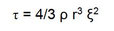
where
τ = the angular deflection in radians
ρ = density of the air
r = the disk radius
ξ = the instantaneous particle velocity of the air.
The Rayleigh disk was a great breakthrough but had very serious functional problems. It could be used only in the laboratory, only under tightly controlled conditions, and solely by well-trained technicians. However, at just the moment the Rayleigh disk was introduced, a group of seemingly unrelated inventions made elsewhere began the process that would bring to a rapid conclusion the era of mechanical sound measurements.
The Electrical Era
Thomas Edison (1847-1931) and Emile Berliner (1851-1929) invented the carbon- button microphone within a week of each other, in 1876. They prosecuted and litigated their priority dispute for a quarter-century. Finally the US Supreme Court upheld Edison’s patent. Edison’s microphone wound up with Western Union. Berliner’s microphone ended up with AT&T, and that microphone will reappear in the history of acoustic measurements.
In 1882, the same year Rayleigh invented his disk apparatus, a French medical doctor, Jacques-Arsène d’Arsonval (1851-1940) was seeking a way to measure the tiny electrical currents inside the human body. He connected a coil of wire to a pivoting needle and placed a large magnet around it. He reasoned that even tiny currents in the coil would deflect the needle. He called this device the galvanometer, the name being homage to Luigi Galvani (1737-1798), who had made a frog’s leg jump in the same way by applying an electric current. So accurate was this creation that d’Arsonval’s galvanometer movement is still the preferred mechanism for analog meters (Figure 5).
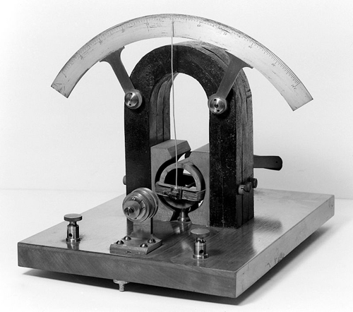
Figure 5. d’Arsonval’s galvanometer was invented for 19th-century medical research (1882) and named after a 17th-century Italian anatomist.
It was George Washington Pierce (1872-l956), obviously an American, who first connected a carbon button microphone to a galvanometer meter movement and measured sound electrically. The carbon button microphone made it a terribly unreliable instrument, susceptible to even minor changes in temperature, humidity, and many thought the phases of the moon. Its fragility and quirks notwithstanding, it simply blew away the mechanical instruments.
The old mechanical instruments would not go quietly into the archives of audio history. Arthur Gordon Webster (1863-1923), remembered for his seminal horn research, wrote in 1919, “I believe I can give more satisfactory answers to all these telephone engineer’s’ queries than can be got by the instruments he gets up by himself. They are handy, no doubt, and all that … [but] I do not do it that way.”
Four Inventions
The electrical era in acoustic measurements really began in earnest in 1917, when Western Electric engineers combined four separate and at the time unrelated inventions to create a machine for practical, reliable sound measurements.
The first was d’Arsonval’s galvanometer, already discussed.
The second was the electrostatic or “condenser” microphone, invented by Edward C. Wente (1889-1972) in 1916. He found that as a charged membrane vibrated, the capacitance between it and a stationary backing plate 220μm away would change according to the deflection. By measuring the undeflected capacitance, the capacitance at a known deflection, and the polarizing voltage, it was elementary to then calibrate the microphone’s electrical output to the diaphragm’s deflection.
But how was Wente to deflect the diaphragm for calibration? His first effort used a closure over the microphone with a small cylinder and piston facing the diaphragm. A rotating motor drove the piston a known stroke length. Unfortunately, the mechanical calibrator worked only at very low frequencies.
For higher frequencies he used the third of our four inventions: the thermophone, devised at about the same time by Harold D. Arnold (1883-1933) and Irving B. Crandall (1890-1927). The thermophone used two strips of gold foil that would vibrate when electric currents were applied to them. To extend the high frequencies available from the thermophone, a flow of hydrogen was introduced into the microphone.
The fourth invention was perhaps the most critical. To amplify the output of the measurement microphone a vacuum tube was employed — we will consider this crucial element in much more detail.
Thomas Edison had discovered what became known as the Edison effect in 1883, through his study of the blackening occurring on the interior of incandescent light bulbs. In 1904 John A. Fleming (1849-1934), a British employee of the Marconi company (and formerly of the British Edison company), used the Edison effect to create the oscillating valve: a vacuum-tube diode.
On 9 December 1905, Lee de Forest (1873-1961) filed a patent on the vacuum-tube triode, which his assistant Clifford D. Babcock had named the audion. By adding a grid to Fleming’s device, de Forest, for the first time, could provide electronic amplification of the signal. In 1912, in Palo Alto, CA, de Forest developed a three-audion amplifier capable of increasing audio-frequency signals by about 120x. He spent almost a year negotiating with AT&T to sell the audion, and finally did so in July 1913.
Edwin Howard Armstrong (1890-1954) demonstrated in early 1913 that the amplifying power of the audion was tremendously increased when part of its output was fed back to the input. This regenerative technique was the subject of ruinous litigation pursued as a holy crusade by both parties until 1934, when the US Supreme Court finally ruled that de Forest was the patent-owner. Nevertheless, AT&T rushed to apply the audion everywhere they could, and in 1915 achieved coast-to-coast telephone transmission using an audion amplifier. Additionally, they were able to broadcast from a radio transmitter in Arlington, Viginia, using 500 audions.
In 1917, AT&T produced a sound-level meter, which along with its many successors were physically huge. In fact, these devices were so cumbersome that in 1988 Leo Beranek (born 1914), in a revision of his classic book [2], described their essential accessories as “a strong back or a rolling table”. Using today’s standards its accuracy was not only questionable, it was transitory.
They were, however, the way acoustic measuring instruments would develop from then on. In 1947 John Bardeen (1908-1991), Walter Brattain (1902-1987), and William Shockley (1910-1989) developed the transistor, and shortly after that the measurement engineer’s weight-lifting talents were no longer required.
The Anechoic Chamber
Until the early 1920s, the vast majority of acoustic measurements were made outdoors to avoid pollution of the data by artificial reflections from the measurement environment.
Researchers and scientists working at Bell Laboratories during the mid-1920s had undertaken to construct an indoor facility to alleviate these problems. A number of rather vague and oblique references to “well-damped measurement chambers” appeared in several Bell publications starting in 1924 and resurfacing occasionally until 1936. In that year E. H. Bedell finally published a paper in the Bell System Technical Journal describing wedges of some kind of fuzz in a former strongroom from which outside sounds and vibrations were excluded. While there is no absolute evidence to support the theory, the lack of published references and vague descriptors used might lead one to suspect these inventors toyed with the idea of keeping the anechoic chamber a trade secret, enabling them to pursue data collection and product development with facilities available to no one else.
What It All Means
Although the long quest in search of reliable measurement has been the beneficiary of a number of happy accidents and serendipitous connections, like many human endeavors, it has also been filled with betrayal and angry controversy. For example, Flamsteed and Halley became estranged from Newton after he caustically and unceremoniously dismissed their measurements as sloppy and then fudged his theory to match similar measurements that couldn’t be denied.
de Forest, the atheist son of a minister, was repeatedly skewered by his fellow scientists and the media as a contradictory self-promoter, an indicted stock swindler, and a would-be inventor-buccaneer. History finds him, variously, the only true begetter of every idea around him, or else a poisonous little toad who stole every idea he saw. Even his surname was a youthful affectation: the lower-case “d” contrived from a family name of De Forest.
During their long litigation de Forest and Armstrong produced hundreds of pages of the most vituperative and scandalous testimony and counterclaims.
Edison and Berliner ended up bitter enemies, and their successor companies spent vast fortunes trying to crush each other.
Our own era has begun to follow a similar path, as we have added another invention to acoustic instrumentation: the computer. The lack of trust many have in the microscopically-focused world of computer-aided measurements is creating a bifurcation that may well once again cause acrimony and stagnation.
It is becoming increasingly obvious that a sizable gap exists between those who trust scientific measurements and those who trust their ears. Some would live and die by the numbers alone. Others would as soon be deaf as judge acoustic and audio system characteristics by only those variables deemed quantifiable by accepted measurements alone.
Essentially these two faiths are separated by a wall of mathematics. Those who subscribe to the objective view of the universe generally require that to quantify a variable, mathematically accurate, repeatable, precise measurements of defined parameters must be made. Electrical and electronic devices are the instruments by which such objective information may be collected. If it cannot be measured or postprocessed then the likelihood of the “information” being of any use is by these standards minimal.
On the other hand, the members of the subjective academy fiercely and vociferously support their contention that, measurements aside, one must also include descriptions of sound couched in terms that illustrate or verbalize sonic or acoustic phenomena and effectively convey these perceived sensations to nonparticipants.
The fulcrum of this debate is how to mathematically and statistically portray the often nebulous or somewhat individualized subjective descriptions, yet maintain a valid scientifically quantified basis for measurement while paying homage to the “art of sound.”
This has rapidly become a complex juggling act.
The issue has surfaced because there are a number of professionals who feel we must be considerably more cautious in accepting the progeny of our microprocessors. The problem is that any computerized system, running any software or generating any measurements we are likely to want or need, is a number-intensive system. It lives and breathes digit after digit, but it knows them not. It cannot tell you that these numbers are right and those are wrong; it simply crunches until some answer appears.
The subjective camp rightfully points out that there still is and probably always will be a subjective factor to all this audio stuff.
We have computers taking measurements and passing them on to other computers with little or no human oversight. We sit mesmerized by our ability to delve into the finest detail, yet we can easily miss the obvious.
To paraphrase the famous nuclear physicist Wolfgang Pauli (1900-1958), measurement technology in the 20th century has become almost like going to the world’s finest French restaurant and being forced to eat the menu.
Richard C. Heyser (1931-1987), architect of time-delay spectrometry and founder of the modern school of mathematically-based audio measurements, offered wisdom on this subject [3]: “Any audio system can be completely measured by impulse response, steady-state frequency response, or selected variations of these such as squarewave, toneburst or shaped pulse … [however, such] measurements will unfortunately always remain unintelligible to the non-technical user of audio systems. … The difficulty lies not with the user, but with the equations and method of test, for these do not use the proper coordinates of description for human identification. … [We] should not expect a one-dimensional audio measurement to be meaningful in portraying an image of sound any more than [we] could expect an art critic to be appreciative of a painting efficiently encoded and drawn on a string.” He added, “… One common-sense fact should be kept in mind: the electrical and acoustic manifestations of audio are what is real. Mathematics (and its implementations) are at best a detailed simulation that we choose to employ to model and predict our observations of the real world. We should not get so impressed with one set of equations (or one measurement format or method) that we assume the universe must also solve these equations or look at things in that particular way, to function. It does not.”
Heyser’s prescient remarks, made four decades ago, are still valid, perhaps even more so given the advancements in measurement hardware and the mathematics that enables it. Beginning with the calculus of long ago, we have moved forward, albeit sometimes haltingly, until as the 21st century opens we have reached a level in measurement technology that enables us to examine, quantify, and supposedly analyze what some practical individuals have dubbed “audio minutia.”
In less than 300 years sound has gone from a mathematic-scientific theory to a tangible quantity we can measure as accurately as, and sometimes more easily than, voltage or resistance.
It is crucial to remember, as we move ever further up the measurement capability ladder, two key facts:
First, it is the non-critical, untrained ear that funds the audio industry. All our customers, and in many cases we ourselves, could care less what the instruments say: Eventually we must all base our critical judgments entirely on what we hear. That enforced psychoacoustic sealing of what is and is not good sound leads us to:
Second, the best and most accurate measurement tool available is free, and it is located on either side of your head. It serves little purpose to measure and quantify the system to the nth degree if your ears tell you it still sounds bad.
In the paper quoted above Heyser also said, “It is … perfectly plausible to expect that a system which has a ‘better’ frequency response, may in fact sound worse simply because the coordinates of … measurement are not those of subjective perception.”
This all comes down to some critical realities:
1. The ability to measure something does not automatically carry with it the ability to understand the measurement’s meaning with respect to aural perception.
2. Machines and microphones do not “hear” in the same way that humans do.
3. The ear-brain system performs subjective analysis. It is also a system wherein the “code” used to process the information is still little understood and the subject of much myth.
4. Just because we can quantify a parameter does not mean we need or can effectively use that data.
5. Despite its lack of scientifically-acceptable facts and mathematically-correct formulas, the subjectively based analysis of perceived acoustic or audio quality is still the measurement system that most sentient residents of this planet accept and understand.
Although our hardware has evolved across the centuries, the user is still a biological entity that sees objects in space and hears events in time. Measurement hardware hears sound as waves, not events. Understanding this distinction is critical, because it focuses on the essential difference between purely logic-based systems and those operating in the biological domain.
The same subjective-objective argument was made about triode tubes versus pentode tubes, and then later about tubes versus transistors. As has been aptly noted [16], “Today’s arguments about distortion, its nature, definition, audibility, and measurement persist. From some of the arguments advanced, this subject will not be resolved soon.”
It is crucial that professional practitioners understand that although objective measurements supply a scientifically valid, thoroughly repeatable data, and must be an integral part of the science of sound, the devices under test will ultimately be used by human beings and not machines. Thus it is also incumbent upon all to accept as equally valid the somewhat less-scientific subjective judgments. After all, it is the biological quality-assessment systems that will be the final judge of our success or failure!
Bibliography
[1] Ampel, Fred, and Ted Uzzle, “The Quality Of Quantification,” Proc. Inst. Acoust., v13 Part 7, pp47-56, 1991.
[2] Beranek, Leo Leslie, Acoustic Measurements, second edition, American Institute of Physics, 1988.
[3] de Forest, Lee, “The Audion Detector And Amplifier,” Inst. Radio Eng. Proc. v2, pp15-36, 1914.
[4] Heyser, Richard L., “The Delay Plane, Objective Analysis Of Subjective Properties: part I,” Jour. Audio Eng. Soc., v21n9, pp690-701, November 1973.
[5] Hunt, Frederick V., Electroacoustics, American Institute of Physics, 1982 (reprint of 1954 edition).
[6] Hunt, Frederick V., Origins in Acoustics, Yale Univ. Press, 1978.
[7] Lewis, Tom, Empire of the Air, Harper-Collins, 1991.
[8] Lindsay, R. Bruce, “Historical Introduction” to Rayleigh, Theory of Sound, Dover, v1, ppv-xxxii, 1945.
[9] Miller, Harry B., editor, Acoustical Measurements, Methods and Instrumentation, Benchmark Papers in Acoustics v16, Hutchinson Ross, 1982.
[10] Newton, Isaac, Principia Mathematica, Univ. of California Press, 1966. His derivation of the speed of sound is in Book Proposition XLIX, pp379-381.
[11] Read, Oliver, and Walter L. Welsh, From Tin Foil to Stereo, second edition, Howard W. Sams, 1976.
[12] Strutt, M. J. O., “Raumakustik,” Handbuck der Experimentalphysik, v17n2, pp443-512, 1934.
[13] Tyndall, John, Sound, Greenwood, 1969 (reprint of the 1903 edition).
[14] Uzzle, Ted, “When The Movies Learned To Talk, part 2,” Boxoffice, v128n5, pp22-23, May 1992.
[15] Uzzle, Ted, and Fred Ampel, “A Brief History Of Acoustical Measurements,” Sound & Video Contractor, v10n5, pp14-22, May 1992.
[16] von Recklinghausen, Daniel R., “Electronic Home Music Reproducing Equipment,” Jour. Audio Eng. Soc., v25n10/11, pp759-771, October/November 1977.