by John Eargle

Editor’s Note:  Written by John Eargle, and republished courtesy of Harman Professional, this article is Chapter 1 of a book he co-authored with Chris Foreman entitled “Audio Engineering for Sound Reinforcement”.  Eargle, who passed away in 2007, was JBL’s Vice President of Engineering for many years and became a well-known author and consultant.  He was a skilled recording engineer responsible for more than 250 CD releases and his work in cinema sound brought him a Technical Oscar in 2001.  Eargle’s many books on audio and acoustics are industry benchmarks and we are pleased to bring Pro Audio Encyclopedia readers this excellent introduction to acoustics.

What is Sound?

For our purposes we will define sound as fluctuations, or variations, in air pressure over the audible range of human hearing. This is normally taken as the frequency range from about 20 cycles per second up to about 20,000 cycles per second. The term hertz (abbreviated Hz) is universally used to indicate cycles per second. Likewise, the term kilohertz (kHz) indicates one-thousand Hz. We can write 20,000 Hz simply as 20 kHz.

A two-to-one frequency ratio is called an octave, a term taken from music notation. For example, the frequency band from 1 kHz to 2 kHz comprises one octave. A frequency decade represents a ten-to-one frequency ratio.

The speed of sound propagation in air at normal temperature is approximately 1130 feet per second (344 meters per second). At higher temperatures the speed of sound increases slightly, while at lower temperatures the speed is less.  The precise values are given by the equations:

(1.1)     Speed of sound in air = 1052 + 1.106 °F feet per second

(1.2)     Speed of sound in air = 331.4 + 0.607 °C meters per second

where temperature is given in both degrees Fahrenheit and Celsius.

Let’s consider the simplest of all sounds, a sine wave. If we take a “snapshot” of one cycle of the sine wave it will appear as shown in Figure 1-1A. Zero on the vertical scale represents normal static atmospheric pressure. We have labeled some important aspects of the wave. The period of the wave is the length of time (in seconds) required for a single cycle, and it is equal to 1/frequency. For example, if we are considering a frequency of 1 kHz the corresponding period will be 1/1000, or 0.001 seconds (1 millisecond).

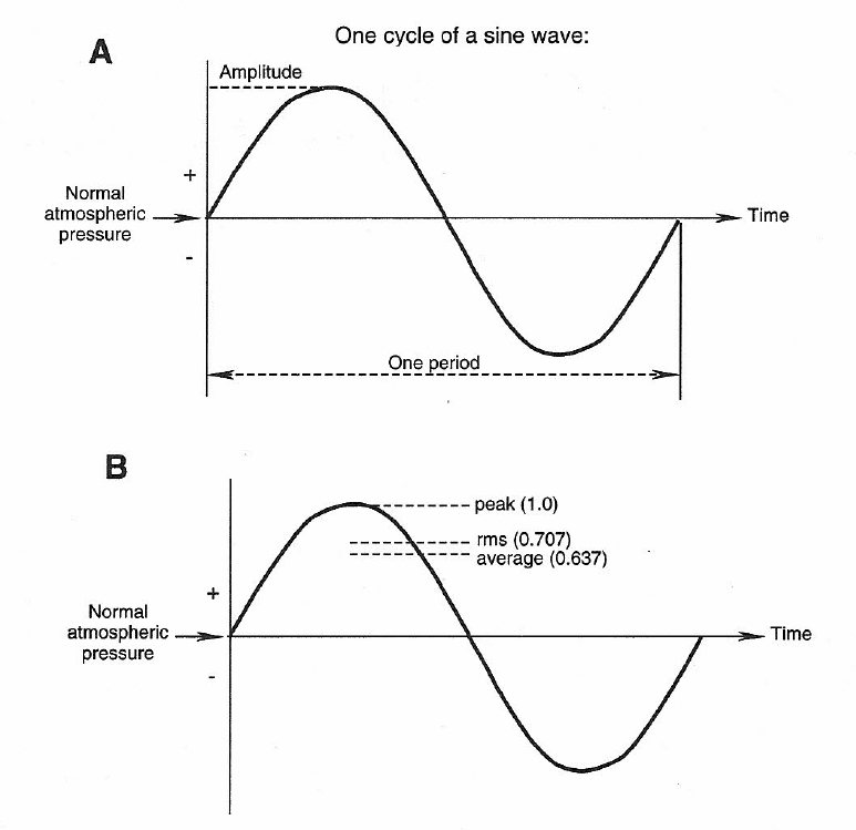
Figures 1-1A & 1-1B: Properties of a sine wave. Definitions (A); peak, rms and average values (B).

As the 1 kHz sound propagates in air, the distance from the start of one cycle to the start of the next cycle will be 1130 divided by 1000, or 1.13 feet (.344 meters). This quantity is known as the wavelength (specifically the wavelength in air). The relationships among speed of propagation (c), frequency (f), and wavelength (λ) are:

c = fλ   f = c/λ   λ = c/f

Another quantity is the magnitude, or the amplitude, of the alternating pressure of the propagating sine wave. While we may measure the static air pressure in a bicycle tire in terms of “pounds per square inch,” acoustics uses the International System (SI) of units in which air pressure is measured in pascals (newtons per square meter). We will discuss this in more detail in a later section.

A sine wave with a maximum amplitude of unity has an rms (root-mean-square) value of 0.707 and an average value of 0.63, as shown in Figure 1-1 B. The average value is simply the value of the signal averaged over one-half cycle, but the rms value gives us the effective steady-state value of the waveform. This is the value that we use in making power calculations, and it is directly proportional to the value that we measure with a sound level meter. Again, these topics will be explained in a later section.

We can envision a sine wave as being generated by the rotating radius of a circle, as shown in Figure 1-2. Two sine waves of the same frequency may be displaced from each other in time, creating a phase relationship between them. As illustrated in Figure 1-3, we can say that one signal leads (or lags) the other by the phase angle ϕ, which we normally state in degrees.

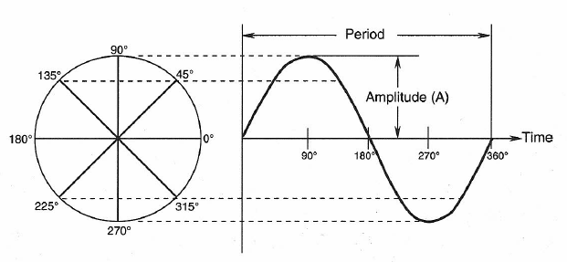
Figure 1-2: Generation of a sine wave with a rotating vector.

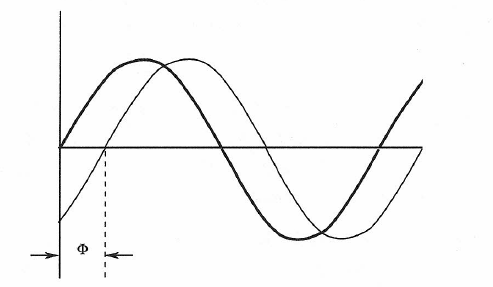
Figure 1-3: Definition of phase relationship between two sine waves of the same frequency.

We can sum displaced sine waves of the same period and, in general, get a new sine wave with a different amplitude and phase angle, as shown in Figure 1-4A. Here, two sine waves of unity amplitude with a phase relationship of 90° combine to produce a new sine wave with an amplitude of 1.4 and a relative phase angle of 45°. In Figure 1-4B two sine waves of the same amplitude with a 180° phase relationship cancel completely if they are summed.

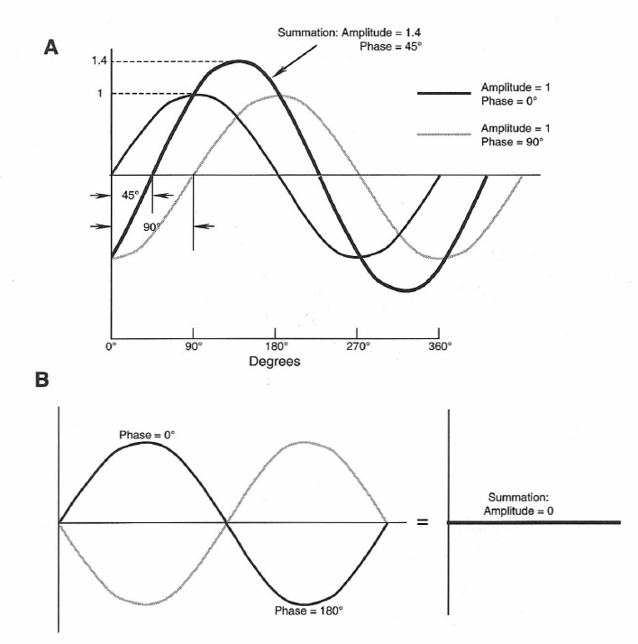
Figure 1-4: Addition (A) and subtraction (B) of sine waves.

Complex Waves

Most musical tones are composed of a set of harmonically related sine waves. If f_o is the fundamental frequency, we can combine it with 2f_o , 3f_o , 4f_o, and so forth, as shown in Figure 1-5, to produce a complex wave. Because the components of the complex wave are periodic multiples of f_o the sum of the harmonics is also periodic.

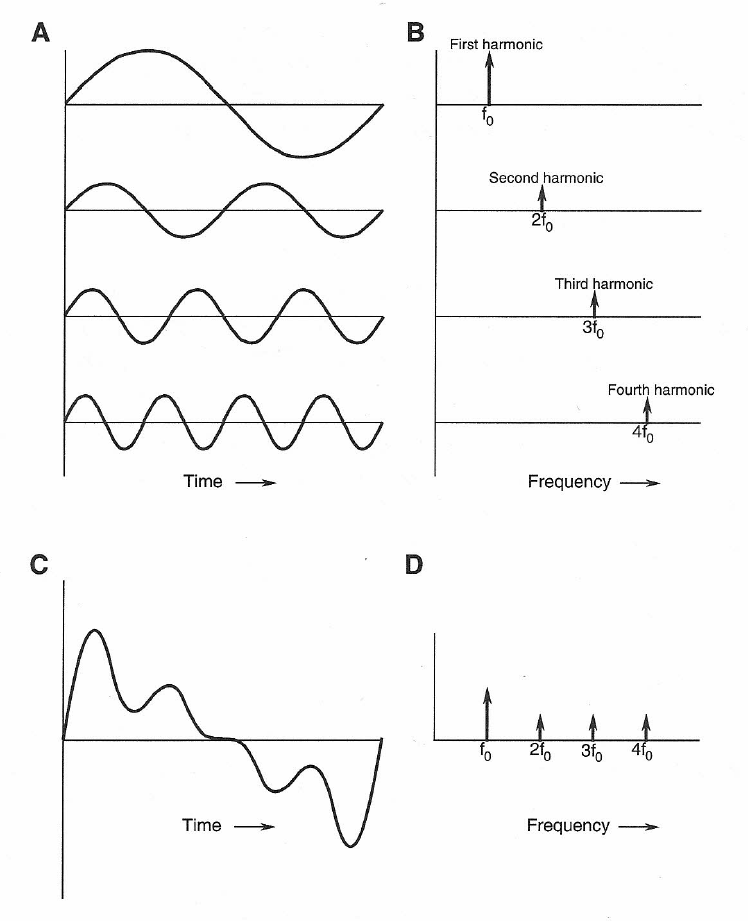
Figure 1-5: Sine wave and harmonics (A); representation of sine waves along the frequency axis (B); summation of harmonically related sine waves (C); representation of summation as values along the frequency axis (D).

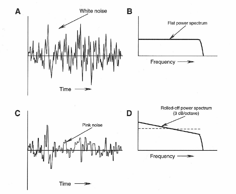
Figure 1-6: White noise: time axis representation (A); frequency axis representation (B). Pink noise: time axis representation (C); frequency axis representation (D).

Diffraction of Sound

Broadly defined, diffraction describes the bending of sound around obstacles in its path. If the obstacle is small relative to the wavelength of the sound, then the sound bends around the obstacle as though it weren’t there, as shown in Figure 1-7A. This is the case when the wavelength is about three-times the diameter of the obstacle or greater.

If the frequency of the incident sound is increased, the wavelength is reduced and the situation becomes more complex. The bulk of the sound will progress around the obstacle, but there will be some degree of reradiation, or back-scattering from the obstacle as shown in Figure 1-7B. In many cases there will be slight changes in sound pressure at the surface of the obstacle as sound makes its path around the obstacle. This situation is what normally happens when the obstacle has a diameter about the same as the wavelength.

If the frequency of the incident sound is further increased, producing even shorter wavelengths, then more sound will be reflected from the obstacle, and there will be a clear shadow zone behind it, as shown in Figure 1-7C. This condition occurs when the diameter of the object is about three-times the wavelength or greater.

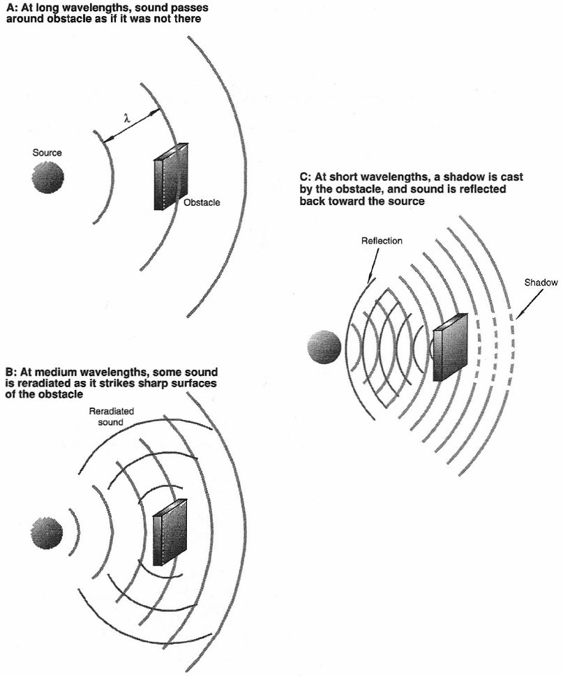
Figure 1-7: Sound waves and obstacles. At long wavelengths (A); at mid wavelengths (B); at short wavelengths (C).

Two further examples of diffraction are shown in Figure 1-8. Sound passing through a small opening in a large barrier tends to reradiate as a new source located at the opening if its wavelength is large relative to the opening. Sound easily goes around corners, as we all know. However, if the sound has a very short wavelength, the discontinuity at the corner will cause some slight reradiation of sound outward from the corner.

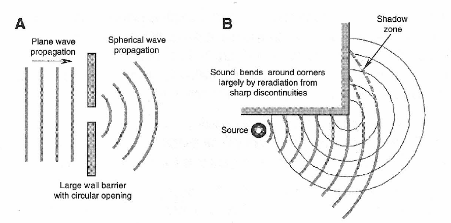
Figure 1-8: Diffraction of sound waves. Spherical reradiation through a small opening in a boundary (A); apparent bending of sound around a corner (B).

Refraction of Sound

Refraction refers to the change in the speed of sound as it progresses from one medium to another, or as it encounters a temperature or velocity change (or gradient) in air out of doors. Several examples are shown in Figure 1-9 and 1-10. These clearly show how, over long distances, sound can appear to skip and shift in direction. A related phenomenon is shown in Figure 1-11, where a strong cross breeze can shift the apparent direction of sound.

Effects such as these are often noticed in large outdoor performance venues, such as the Hollywood Bowl, where large sloped natural surfaces favor the development of upward thermal wind currents.

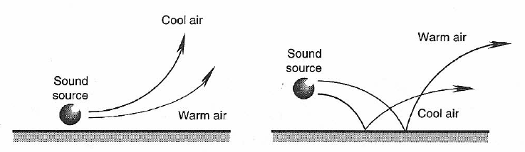
Figure 1-9: Effects of temperature gradients on sound propagation.

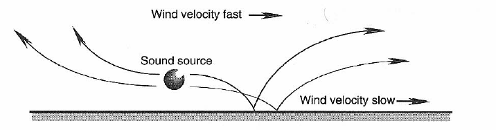
Figure 1-10: Effects of wind velocity gradients on sound propagation.

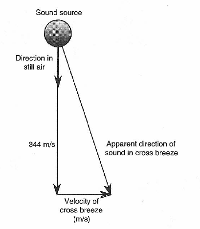
Figure 1-11: Effect of cross-wind on sound propagation direction.

Reflection, Absorption, and Transmission of Sound at a Barrier

Figure 1-12 shows a typical wall separating adjacent rooms. Sound that strikes the wall goes in several directions. Most of it is reflected back into the room where the sound originates. Some of it is absorbed internally in the wall structure and converted to heat, and a relatively small portion is transmitted through to the other side.

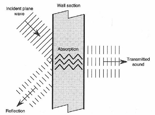
Figure 1-12: Sound at barrier: reflection, absorption and transmission through boundary.

There is little that we can do after the wall has been built to improve isolation (reduce transmission) between adjacent rooms, since those characteristics are inherent in the design and construction of the wall. However, what we can do is increase absorption at the surface and reduce reflections coming back into the originating room. This can take the form of simple externally applied damping materials, such as fiberglass battens or multiple folds of heavy drapery. Later, we will see how we can mount the damping material to give the maximum amount of absorption at a given frequency.

The reflection of sound from a wall normally involves some degree of scattering. In Figure 1-13A we see what happens when sound of a fairly short wavelength strikes an absorptive surface at an oblique angle. Most of the sound is absorbed, but some rebounds at an angle equal to the angle of incidence. In Figure 1-13B we see what happens when the wall surface has very little absorption; most of the rebounding sound is concentrated at the complementary angle, but some is reradiated at adjacent angles.

We also know that sound striking irregular surfaces tends to scatter to a large degree. When the surface has been mathematically designed to maximize this effect, as in Figure 1-13C, the sound is essentially reradiated in all directions in the plane of reflection. The specific diffusing surface illustrated here is the quadratic residue diffuser (Schroeder, 1984; D’Antonio, 1984).

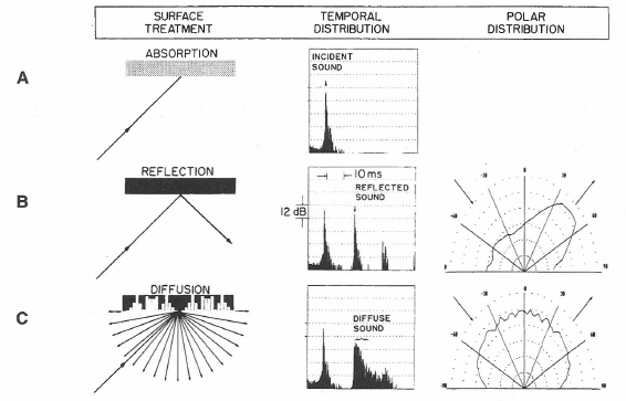
Figure 1-13: Sound reflection at a boundary absorption, specular reflection and diffusion. (Data courtesy RPG Diffusor Systems, Inc.)

Definition of Absorption Coefficient

Acousticians use the term absorption coefficient to describe the ratio of acoustical power absorbed to the total sound striking a boundary. For example, a surface with an absorption coefficient of 0.3 will reflect 0.7 of the power and absorb the remaining fraction of 0.3. If the surface has an absorption coefficient of 0.1, it will absorb 10% of the power and reflect the remaining 90%. The sound power that is absorbed at the boundary merely becomes heat; normally, some of the power is transmitted through the boundary and is reradiated as sound on the other side of that boundary.

Absorption coefficients normally range between zero (no absorption) and 1 (total absorption), and published values for many materials and surface finishes are given in acoustical handbooks over several octave bandwidths covering the range from 125 Hz to 8 kHz. The Greek symbol alpha, α, is used to indicate an absorption coefficient. The concept will be expanded in a later section of this chapter.

How We Measure Sound: The Decibel (dB)

When we speak only in terms of sound pressure, we are dealing with numbers which, from the softest audible sounds to the loudest, cover a million-to-one ratio. This would involve some rather large and clumsy numbers, and in the early days of telephone research, mathematicians simplified the notation with the introduction of the bel and the decibel. In using decibels we are expressing the level of one signal with respect to another (the term level is exclusively used in audio engineering for ratios given in dB).

(1.3)     bel = 10 log₁₀ (W/W₀)

where W₀ is a reference power and W is any other power. For example, let our reference power be one watt and let W = 10 watts. Then:

Ratio in bels = 10 log (10/1) = 1 bel

We can state that the level of 10 watts relative to one watt is 1 bel.

For more convenient scaling of the numbers, we more commonly use the decibel, which is defined as:

(1.4)     Ratio in dB = 10 log (W/W₀)

and in this case the ratio is: 10 log (10/1) = 10 dB

From this basic definition we can construct the following chart which gives the level in dB for various powers, all referenced to one watt:

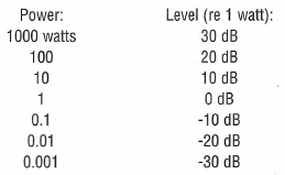
Here, the range of power values is a million-to-one; using levels in dB, we have reduced this numerical range to a far more convenient 50-to-one range. Figure 1-14 presents a convenient nomograph that lets us read the decibel level directly between any two power values over the range given above.

A given difference in dB always corresponds to a given ratio in power. For instance, a 2-to-1 ratio in power always represents a 3 dB change in level. Look carefully at Figure 1-14; pick any pair of powers with a 2-to-1 ratio, then carefully read the difference in dB directly adjacent on the scale and you will see that the difference is always 3 dB. For example, locate 40 and 80 on the power (watt) scale; looking at the adjacent levels we read 16 and 19 dB. Thus, 19 -16 = 3 dB.

Note also that any 10-to-1 power ratio is always represented by a 10 dB difference in level.

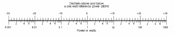
Figure 1-14: Nomograph for relating power in watts with level values in dB.

Relating the Decibel to Sound Pressure

We do not normally measure sound power; instead, we measure rms sound pressure using a sound level meter (SLM), which is calibrated directly in dB. You can spend several thousand dollars for a precision SLM, but for many applications a low cost SLM from your corner electronics store will suffice.

Acoustical power is proportional to the square of sound pressure; therefore, doubling the sound pressure will produce a quadrupling of acoustical power. As we have seen, doubling power represents a 3-dB level increase; doubling it again will add another 3 dB, making 6 dB. Therefore, we can construct a new scale in which a doubling of sound pressure corresponds to a 6-dB increase in sound pressure level (SPL), and a 10-times increase in sound pressure corresponds to a 20 dB increase in SPL. This new scale is shown in Figure 1-15A. The “zero” dB reference pressure for this scale has been chosen as 20 micropascals, which is the threshold of hearing in the 3 to 4 kHz range for persons with normal hearing. A photograph of a professional sound level meter is shown in Figure 1-15B. The chart shown in Figure 1-16 shows typical sound pressure levels encountered in everyday life.

A more thorough treatment of the decibel is given in Appendix 2 at the end of this book.

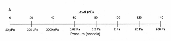
Figure 1-15A: Relation between dB SPL and pascals.

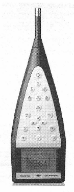
Figure 1-15B: Photo of a digital sound level meter (photo courtesy B&K).

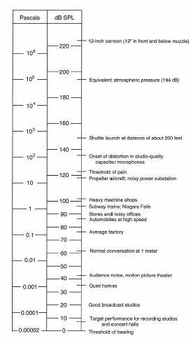
Figure 1-16: Sound pressure levels of common sources.

A Free, Progressive Sound Wave: Inverse Square Law

Consider a small sound source outdoors located away from any reflecting surfaces and emitting a continuous signal. We will measure the sound pressure at some reference distance d and detect a pressure value of p₁. Now, if we move to a distance which is twice d, we will detect a new pressure value, p₂, which will be one-half of p₁. This process may be carried out indefinitely, with each doubling of distance producing a halving of pressure. The process is shown in Figure 1-17.

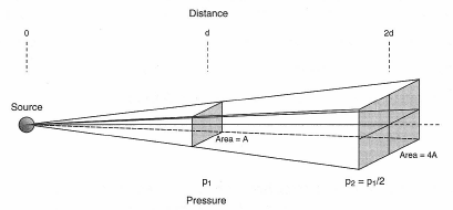
Figure 1-17: Illustration of inverse square law.

At distance d in Figure 1-17 we show an area through which passes a certain amount of radiated sound power. At a distance of 2d, that same power is now radiated through four-times the original area. The relationship of quadrupling the number of squares for the doubling of distance is referred to as the inverse square law.

The halving of sound pressure at distance 2d represents a drop in sound pressure level of 6 dB relative to distance d, and we can now construct a new nomograph for determining sound pressure levels as they vary with distance from a source in a reflection-free environment (so-called free space). The new nomograph is shown in Figure 1-18. In order to show the correspondence between doubling distance and reducing the level by 6 dB, we must plot 20 log (D/D₀), where D₀ is our reference distance of one foot (or one meter).

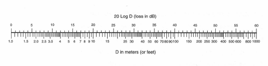
Figure 1-18: Nomograph for relating inverse square level loss in dB with distance from sound source.

As an example of using this nomograph, let us assume that a given source produces a sound pressure level of 94 dB at a distance of one meter. What will the level be at a distance of 20 meters? Referring to the nomograph, locate the distance 20 on the foot (meter) scale. Directly adjacent to 20 read 26 dB. The level will then be 94 – 26 = 68 dB SPL.

In addition to level losses over distance due to the inverse square effect, there is additional loss at high frequencies due to air absorption. An indication of this is shown in Figure 1-19. Along the left vertical axis, you will note the excess attenuation in dB per 100 feet (30 meters) encountered over long distances. Note the high dependence on relative humidity; high frequency losses are greatest when relative humidity is in the range of 20% and least when relative humidity is high.

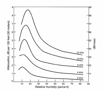
Figure 1-19: Excess loss with distance due to relative humidity in air.

As an example of air losses at high frequencies when relative humidity is 30%, let us calculate the loss in dB between distances of 2 feet and 200 feet from a source. At low frequencies, below about 500 Hz, only the inverse square loss will be significant. Using the nomograph in Figure 1-18, we can see that the loss will be 40 dB. For a frequency of 10kHz, there will be an additional loss due to absorption in the air itself. From Figure 1-19 we can read the loss per 100 feet at 30% relative humidity as about 5.5 dB. So the total excess loss at 10 kHz would be very close to 11 dB over the distance from 2 feet to 200 feet. Adding this to 40 dB gives a total loss at 10kHz of about 51 dB.

Nearfield and Farfield Considerations

If we make measurements too close to a typical sound source, we may not get the answers we would expect according to the discussion given above. Typically, if we are closer to a source than about 5-times its greatest dimension, we are in its near field. Beyond that distance we are effectively in the far field. Note of course that there is no exact point where we leave one and go into the other; there is rather a transition range between the two.

Summing Levels in dB

Assume that a point source of sound has a level of 94 dB SPL at a given distance. Now, let us add another point source with the same 94 dB level, again at the same distance. What will be the resulting sum of the two? Since both sounds are individually of the same level, their acoustical powers will be equal, and we will effectively be doubling that power when both are sounded together. This represents an increase of 3 dB, making a resultant level of 97 dB.

Let’s now do another experiment: Assume that we have an existing sound pressure level of 94 dB; we want to add to it another sound pressure level that is only 84 dB. What will be the new level? This is a little more complicated, and we proceed in five steps as follows:

1. Let’s assign an arbitrary power to the first level (94 dB) of one watt.
2. Since the second level (84 dB) is 10 dB lower, it has as power of 0.1 watt.
3. Now, we add the two powers and come up with a sum of 1.1 watts.
4. Taking 10 log (1.1), we come up with an incremental level of 0.4 dB.
5. Therefore, the resultant overall level is 94 + .4 = 94.4 dB SPL.

There is a simple way to arrive at this answer, and it is given by the nomograph shown in Figure 1-20. Here, D is the difference in dB between the two levels. Read directly below D to obtain a number N; N is then added directly to the higher of the two original levels to arrive at the sum of the two.

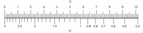
Figure 1-20: Level summation of two sound power sources.

Let’s rework the previous example using the nomograph. Taking the original 10-dB difference as D, we read the value of just slightly higher than 0.4 for the corresponding value of N. We then add that to 94 and get the answer of 94.4 dB.

Directivity of Sound Sources

Many sound sources have radiation patterns that favor one direction. A trumpet, for example has directivity that is maximum along the axis of its bell, and a talker has directivity that is largely maximum in the forward direction. Loudspeakers that are used in sound reinforcement are likewise designed for maximum radiation within a clearly defined solid angle so that reinforced sound may be directed where it is needed.

The basic presentation of directivity information is by way of the polar plot, in which the response of a device, under fixed signal excitation, is measured as it is rotated over a 360-degree angle in a single plane. An example of this is Figure 1-21, which shows the polar response of the spoken voice in both vertical and horizontal planes. A separate polar plot must be made for each frequency or frequency band of interest.

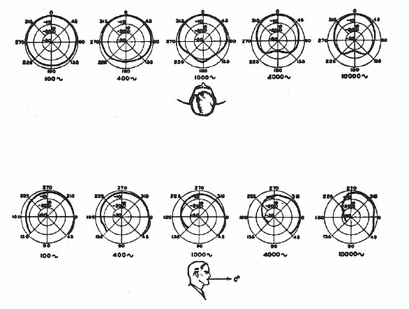
Figure 1-21: Directivity of the human voice in horizontal and vertical planes (Olson, 1957).

There are many methods for presenting directivity information, and some of them are shown in Figure 1-22. Frontal isobars are shown at A; here, the -3, -6, -9, and -12 isobars are plotted in spherical coordinates as seen along the polar axis of a globe. A great deal of polar data must be measured in order to make such a detailed presentation as this.

Off-axis frequency response curves, as shown at B, are useful in detailing the response of a loudspeaker over its normal frontal horizontal coverage zone.

For many design applications, simple plots showing the angular spread between the -6-dB response angles in the horizontal and vertical planes are quite useful, as shown at C.

Finally, the plot of directivity index (DI) in dB is shown at D. DI is probably the most useful qualifier of directivity performance and involves only a single numerical value at each measurement frequency. DI is defined graphically in Figure 1-23. It is the ratio of sound level along a selected axis of a radiating device to the level that would exist at that measurement distance if the same acoustical power were radiated uniformly in all directions.

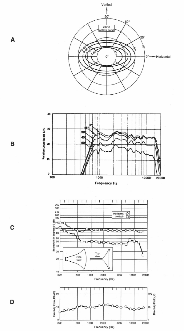
Figure 1-22: Loudspeaker directivity shown as frontal isobars in spherical coordinates (A); as a set of off-axis frequency response curves (B); as a set of horizontal and vertical-6-dB beam width plots (C); and as a plot of on-axis directivity index (DI) and directivity factor (Q).

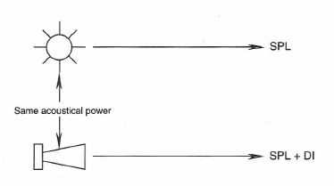
Figure 1-23: A graphical definition of directivity index of a loudspeaker.

Directivity factor (Q) is another way of considering the same ratio. The relationship between DI and Q is given by:

(1.5)     DI = 10 log (Q)           Q = 10^DI/10

The values of both Q and DI are used in audio engineering. Q represents a ratio, while DI is that same ratio expressed in dB.

The Indoor Sound Field

The behavior of sound indoors is fairly complex, but fortunately there are a number of simplifying assumptions that make the analysis much easier. When a steady sound source is turned on in a room, there is first a short time period during which the sound reaches all parts of the space and establishes a steady-state condition.

When this condition has been reached, sound power is absorbed at the room boundaries at the same rate at which it is emitted by the source. After the steady-state condition has been reached, let the sound source be turned off. We then observe that sound in the room dies out after some short period of time. Figure 1-24 shows the nature of the buildup and eventual decay of sound in the room. The curve shown at A describes the variation in sound pressure, while the curve shown at B describes the build-up and decay processes in terms of level. The process shown at B is in fact the way we hear the sound rise and decay, since our hearing is essentially exponential in response.

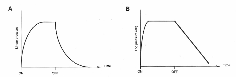
Figure 1-24: Buildup and decay of sound in a live room. Variation in sound pressure (A); variation in sound pressure level (B).

We might think of many individual “rays” of sound, each going its own way from the source in a different direction. Statistically, it can be shown that the average distance (mean free path) a ray of sound travels in the room between successive encounters with boundaries is given by:

(1.6)     Mean free path = 4V/S

where V is the room volume and S is the total area of the room boundaries. (The equation holds with either English or metric units.) This process is shown in Figure 1-25. While each surface in the room may have its own absorption coefficient, α, there will effectively be, after several reflections through the room, an average absorption coefficient, which we designate as α.

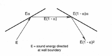
Figure 1-25: Reflections and absorption of sound at two successive room boundaries.

The Reverberant Field and Reverberation Time

After the sound source has been turned off, we will hear a relatively smooth decay of sound in the room. The length of time it takes for the sound to decay 60 dB after the power source has been turned off is known as the reverberation time and is an important qualifier for music or speech perception in any space. The Sabine equation gives a fairly accurate estimate of reverberation time in fairly “live” spaces, those in which the average absorption is no greater than about 0.25:

(1.7)     Reverberation time (seconds):

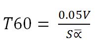
where V is the room volume in cubic feet, S is the room boundary area in square feet, and alpha-bar is the average absorption coefficient in the room.

In metric units the equation is:

(1.8)     Reverberation time (seconds):

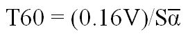
where V is the room volume in cubic meters and S is the room boundary area in square meters.  Alpha-bar will be the same in both cases.

We can measure reverberation time today with any number of acoustical data gathering and analysis programs for personal computers. If we have enough data on the room’s physical aspects, we can calculate it by estimating the room volume, surface area, and deriving the average absorption coefficient as follows:

(1.9)     Average Absorption Coefficient

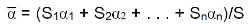
where S₁, S₂, … S_n represent individual surfaces in the room and α₁, α₂ … α_n represent their respective absorption coefficients. S is the total boundary surface area of the room. The unit of absorption is the sabin and is equivalent to one square foot (or square meter in the SI system) of totally absorptive surface area. There are other equations for reverberation time, but none as useful and simple as the Sabine equation used here. See Appendix 3 for further discussion of reverberation time equations and calculations.

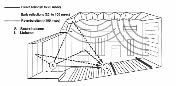
Direct, Developing, and Decaying Sound Fields in a Room

Now, let’s replace the steady source of sound with a short impulsive one and see how sound develops in the room. In Figure 1-26 we see what happens during the first 25 milliseconds (msec) or so after an impulsive sound has taken place on stage. At first, only the direct sound reaches the listener. Then, during the next interval (25 to 100 msec) a volley of discrete, developing reflections will reach the listener, most of them arriving from the front and sides of the room. Finally, beyond 100 msec, decaying sound will arrive from all directions in the room more or less equally.

Figure 1-26: Direct, early reflections and reverberation of sound in an auditorium.

The time response as heard by the listener is shown in Figure 1-27. Here, we can identify the initial time delay (ITD), that short period of time after the arrival of the direct sound, but before the first reflection arrives. In most moderate size listening spaces this gap is about 25 msec. Acousticians often speak of the early sound field, which exists up to approximately 100 msec after the arrival of direct sound. It is important in that it adds loudness and a sense of spaciousness to music presented in the room. If the early sound field is too loud, as may be the case in small, live rooms, the listener may be bothered by blurring and “smearing” of musical and speech details.

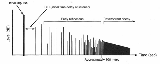
Figure 1-27: Time behavior of sound reflections in a room as measured at a listening position.

Reverberation, including early and decaying sound, often enhances music but is beneficial for speech only when it is fairly short. One of our main jobs in sound reinforcement design is to minimize the effect of the reverberant field without actually reducing it.

Sound Attenuation with Distance Indoors

Figure 1-28 shows what happens indoors as a listener moves away from a sound source. We have labeled the direct sound attenuation curve, and we see that it continues to fall off in level 6 dB per doubling of distance away from the source. The reverberant level is substantially constant throughout the room.

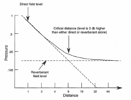
Figure 1-28: Relation between direct sound field and reverberant sound field in a room.

Critical Distance

A good experiment is to have a friend stand in a fixed position in a moderately live room and talk in a clear voice. Your job is to listen at gradually increasing distances. Face the talker as you slowly move away.

The direct sound from the talker will attenuate fairly quickly at first, and you will find that, with a little practice, you will be able to identify the zone where the direct sound from the talker and the reverberant sound in the room are about equal. This happens at a point known as critical distance, D_c. A good way to “zero in” on critical distance is to start close to the talker, moving away until you hear both direct and reverberant sound about equally. Then, beginning far away, walk toward the talker – again identifying the spot where both components sound about equal. Chances are that you won’t be far off, either way.

We can determine critical distance fairly accurately from what we know about the room and the nature of the talker. The equation for determining critical distance is:

(1.10)     Critical Distance

where Q is the directivity factor for the sound source in the direction of observation, S is the surface area in the room, and alpha-bar is the average absorption coefficient for the room.

All of these quantities are known to us: both S and alpha-bar have been discussed and can be arrived at either through direct measurement or calculation. Q was discussed earlier. The nominal Q for the spoken voice in the middle of the articulation range is about 2 (corresponding to DI = 3 dB).

At D_c, both direct and reverberant fields have the same value; therefore, the level (power summation) at D_c will be three dB greater than either field alone. At a distance of 2 D_c, the direct field will be just a little more than 6 dB below that of the combined fields, and at a distance of 4 D_c the direct field will be 12 dB below the combined fields.

We will see in the next chapter how the quantities of reverberation time and direct-to-reverberant ratio play principal roles in estimating the intelligibility and effectiveness of speech reinforcement systems.

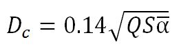
Increasing the Direct-to-Reverberant Ratio

We can increase the direct-to-reverberant ratio in the listening space by increasing D_c. We can do this in two ways: increase the value of α̅ or increase the value of Q. Figure 1-29 shows the effect of increasing room absorption. Note that as the amount of absorption in the room increases, the intersection point (critical distance) between the direct field value and the reverberant value moves to a greater distance.

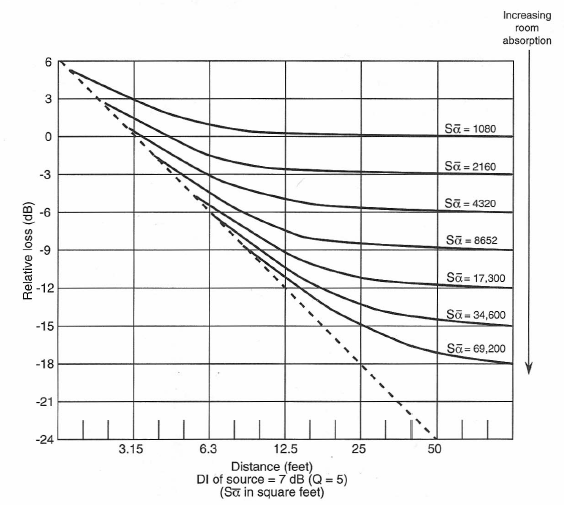
Figure 1-29: Effect of increasing absorption (room constant) on reverberant level with distance in a room.

Figure 1-30 shows the effect of keeping the absorption in the room constant while using a sound source with a higher value of directivity. The increase in source directivity produces more “reach” than that of a lower directivity radiator, and the value of D_c is again increased.

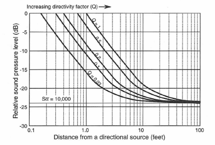
Figure 1-30: Effect of increasing source directivity on direct field level with distance in a room.

Standing Waves in Small Rooms

Our last topic in this chapter will deal with an acoustical wave phenomenon encountered in all spaces, but particularly bothersome in small rectangular spaces. A standing wave may be set up between two parallel walls when there is a sound source located between them. The lowest standing wave between the parallel walls takes place at the frequency whose half wavelength is equal to the distance between the walls. This is shown in Figure 1-31, where x = λ/2. Additional standing waves will take place at higher integral multiples of this number.

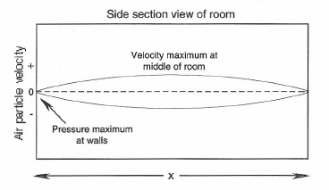
Figure 1-31: A standing wave between parallel walls in a room.

The pressure and air particle velocity distribution in the standing wave is such that at the wall boundary the pressure is at a maximum and the velocity at a minimum. Conversely, at the middle of the standing wave, where the distance from the wall is equal to λ/4, the velocity is at a maximum and the pressure is at a minimum. In Section 1.6 we mentioned that it was possible to place sound absorbing materials for maximum sound absorption at a wall. This distance is precisely at the λ/4 position, as shown in Figure 1-32. When located at a distance that corresponds to a quarter wavelength at some chosen frequency, the high air particle velocity through the damping material will result in maximum sound absorption for that frequency and for its higher odd multiples.

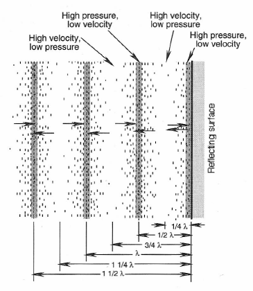
Figure 1-32: Distribution of air pressure and particle velocity near a reflecting surface in a room.

Three-Dimensional Standing Waves, or Room Modes

Any three-dimensional enclosure will support a family of standing waves. Those in a rectangular enclosure are the easiest to calculate and are given by the following equation:

(1.11)     Room Modes

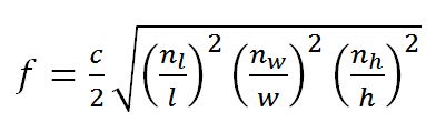
where c is the speed of sound; l, w, and h are respectively the length, width, and height of the rectangular room, and n_l, n_w, and n_h are independent integers.

As an example of three-dimensional mode structure we show the data of Figure 1-33 for a room with dimensions of 6 by 4 by 10 meters. Here, we observe the response of a loudspeaker placed in one corner of the room as it is fed a swept sine wave signal. As you can see, at a frequency about ten-times that of the lowest room mode, the modal density is fairly uniform.

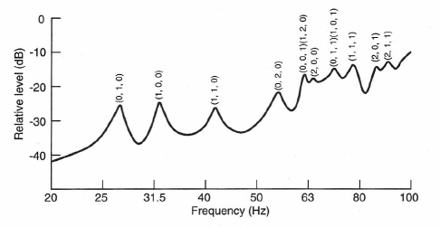
Figure 1-33: Typical distribution of three-dimensional room modes at low frequencies.

In large spaces, room modes are already very dense at frequencies as low as 25 or 30 Hz, and their presence is an essential ingredient in reverberation. It is only in relatively undamped small rooms that individual modes may be troublesome and call for selective absorption at the room boundaries.